
Speed Up Feature Engineering for Recommendation Systems
At Snap, we have a strong focus on user experience and have built many ML applications to surface the right content to our users. Historically, our engineers have spent a significant amount of time working with features. We’ve found that by automating the creation and consumption of a few common features types, we can simplify the majority of feature engineering work. This provides an opportunity for building a general-purpose feature platform that benefits many business critical ML use cases.

Every machine learning model needs input data for training and predictions. Feature engineering is the process of leveraging prior knowledge of the raw data and representing it in a manner that better facilitates learning. While deep learning advancements have largely removed the need for explicit feature engineering in computer vision and NLP, feature engineering remains a crucial component in recommendation systems.
At Snap, we have a strong focus on user experience and have built many ML applications to surface the right content to our users. Historically, our engineers have spent a significant amount of time working with features. We’ve found that by automating the creation and consumption of a few common features types, we can simplify the majority of feature engineering work. This provides an opportunity for building a general-purpose feature platform that benefits many business critical ML use cases.
We present Robusta: our in-house feature platform, built to streamline and accelerate ML iteration.
Extracting modeling signals had been a high friction activity for many Snap teams. Historically, teams solely relied on a forward-fill process that requires implementing and logging features in critical service components. Then, they wait for feature logs for weeks before training any model.
Over time, this process proved to be a major bottleneck:
ML engineers are generally not familiar with online serving components, touching them is risky. On the other hand, delegating to infrastructure engineers introduces coordination overhead.
The turnaround time to tell whether a feature is useful or not is extremely long.
Each team builds their own infrastructure with overlapping functionalities. While teams with more engineering resources can build more sophisticated systems, smaller teams don’t have easy access to more advanced features. Besides, it’s almost impossible to share features.
It was under this context that we started to ask ourselves: can we make ML feature engineering easier?
The feature automation framework Robusta (named after a coffee bean) is our initial attempt to address the pain points. It focuses on associative and commutative aggregation features. These features are widely used in our ML applications, sometimes accounting for more than 80% of the signals in an ML model. The associative and commutative properties are very friendly to distributed systems and allow us to make convenient assumptions. In fact, many companies in the industry have similar systems, e.g. Airbnb Zipline [1] and Uber Palette [2]. We took great inspiration from them.
We have a clear picture of what Robusta should look like. Namely, we want a unified framework that allows ML engineers to easily define features using any engagement data they have access to and share between teams; features can be updated with near-realtime cadence; in addition to forward fill, we must support offline feature generation to unblock quick experimentation with features.
While designing and implementing Robusta, some notable challenges we have to overcome are:
Velocity: How to enable new features end to end through a single declarative feature specification, without manual service deployment and without imposing risks to ML infrastructure.
Scale: A typical ML use case has thousands of aggregation features with varying properties. For example, they could have different sliding windows, sometimes aggregated by user id, sometimes by snap id, or a combination of multiple keys (i.e. user id + discover channel + hour of day). There are operations that can be easily expressed as associative and commutative operations, while also operations that require some work to tweak and fit. We need to design a framework that allows for these possibilities while running efficiently on billions of events per day.
Correctness: How to support offline generation of near-real time features, aka solving the so-called point in time correctness problem [3]. We must answer what the feature value was at online inference time. This is especially challenging when we have sliding window features that can be updated at minute level granularity, as the feature value could be changing every minute for most users as time goes by even without any new engagement events.
We will dive into these problems in the following sections.
Robusta features are built on top of associative and commutative operations. This fundamental assumption is what enables Robusta to perform any number of aggregations efficiently and at scale. If the operator is associative, we can group a subset of elements arbitrarily and that won’t change the outcome; if it’s commutative, the order of the sequence does not matter.
Having these properties allow our system to model the data operation with three basic functions (a similar concept can be found in many data processing frameworks, e.g. MapReduce [4], apache beam [5]):
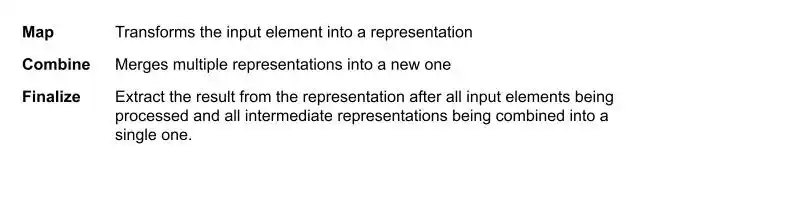
Many operations in ML signal extraction can be expressed with the above functions, such as count, sum, approximate quantiles, etc.
In fact, we can model any data operation if we have a representation that can accurately/approximately restore each input element. For example, trivially:
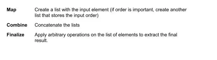
This could still be useful because a lot of signals in recommendation systems are quite sparse, especially at the user level(i.e. sharing a snap). It’s feasible to capture rich contextual information for each sparse event in a list. This list can be either passed into the modeling layer directly or undergone some processing at the finalized step. In other cases, this list approach can be just a starting point for modeling features as associative and commutative operations. We continue to optimize the representation until it’s feasible.
Many ML features require getting the counter for a time range starting from now. This could be challenging since the counter value could change as time goes by even without any new incoming events. Decomposability of the stats makes it convenient to calculate the value for any sliding window at any point in time.
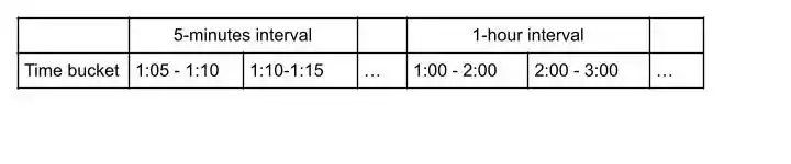
For most stats, we precompute and store intermediate representations for a hierarchy of time ranges. Later on, we will assemble these pre-aggregated blocks to obtain the final stat value for a sliding window, as shown in figure 1.
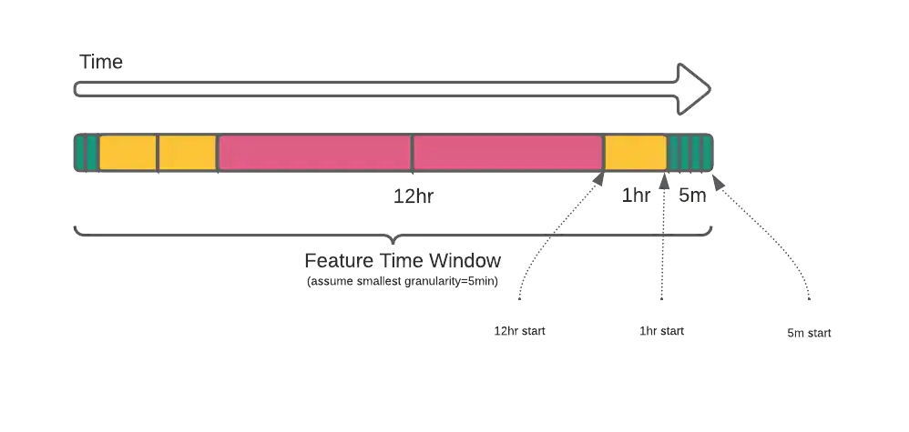
Figure 1. Pre-aggregated blocks in a sliding window
For example, to get the feature value for 5/5 1:14pm with a 24-hours sliding window, we can assemble the following blocks:
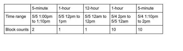
Note that the original timestamp is rounded down to be aligned with the smallest granularity, i.e. 5-minute. Assume duration of each granularity is composed of M smaller granularities (i.e. 1-hour has twelve 5-min granularities) and if we use N consecutive granularities, we need to combine ((M-1) * N - 1) times to assemble all the blocks in the worst case.
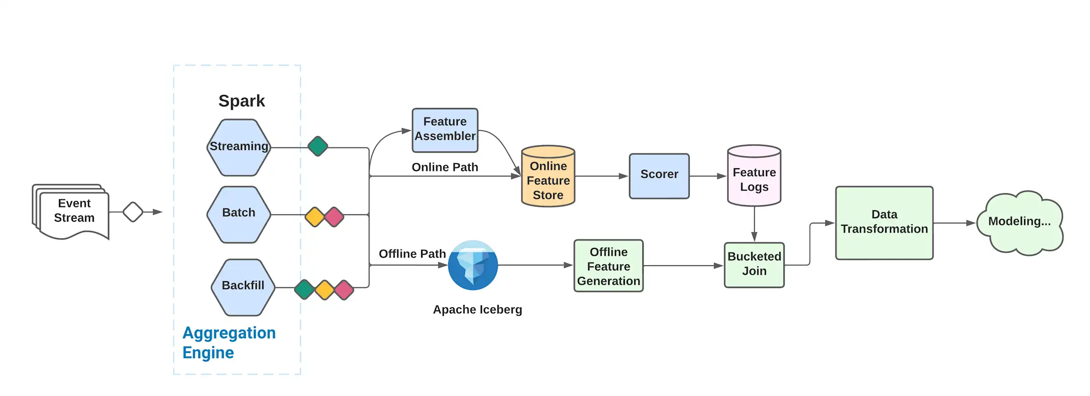
Figure 2. System architecture
The above diagram is the system architecture. The aggregation engine running on dataproc Spark [6] produces data representations for different aggregation granularities. We use a streaming + batch lambda architecture. The streaming component emits data with minute level frequency and ensures freshness of the data; the batch component emits with hour/day level frequency and ensures completeness of the data.
The pre-aggregated blocks will be written to an apache iceberg table [7]. We can use this data to generate features offline, allowing for fast feature experimentations with no dependency on forward-fill.
For online serving we either directly write the blocks for different aggregation granularities to the feature store and assemble them at scoring time, or we preassemble offline. We have the flexibility to switch between the two modes based on use case.
There are also two ways to produce Robusta features offline for training. The modeling team can choose to log them (forward fill) or generate offline. The latter approach is usually taken for experimental features or features that are expensive to store. We implemented a bucketed join algorithm to efficiently join these different feature sources.
ML engineers can specify the feature aggregations they want with a yaml config file:
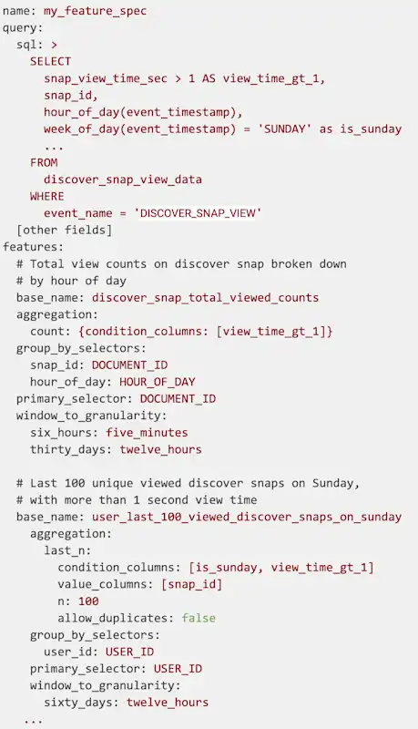
Figure 3. Feature Config Example
Figure 3 is an example. The config consists of two parts:
A SQL statement to apply data processing such as column transformations, row filtering or deduplication.
Aggregation definition that references columns in the SQL statement.
The query section is a SQL that transforms the input data. Columns in the SELECT statement can be used as input to the aggregations in the features section. The FROM statement references a predefined data source in Spark implemented by customer teams.
We chose to have a separate features aggregation section(similar to [1]) in addition to the SQL because different features could have different aggregation keys and it’s very hard to express them all in a single SQL statement. Aggregations are referred to as base features since each one can produce multiple features. For example, discover_snap_total_viewed_counts in the example has two windows(six_hours, thirty_days) attached to it corresponding to two features.
The group_by_selectors field defines the group by keys for the aggregation. This is a mapping from input column name to an enum. In different contexts, the enum pins the data to a particular semantic concept. For example, “snap_id” in the input data is pinned to the DOCUMENT_ID concept; at serving time we need the same id to look up data and it might have a different name such as “id”. Lastly, the primary_selector field defines what should be the primary key for the base feature.
We employ a typical lambda architecture for the aggregation pipelines. Both the streaming and batch jobs run in Spark. The streaming job is responsible for producing minute-level pre-aggregations, while the batch job handles >=1hr aggregation intervals. For even larger intervals such as one-week, we roll up smaller intervals.
Customers can implement their own data source in Spark using the Dataset API. Once the data is loaded, we use Spark SQL to apply the SQL query in the feature spec.
After the SQL transform, the job usually needs to handle hundreds of aggregations. These aggregations execute the map and combine functions discussed earlier. The results are representation blocks for various intervals. They can be assembled to obtain a final feature value later.
At this point we only have the intermediate representations. They might reside in a key value store such as Aerospike for easy point look up or in Apache Iceberg tables for high throughput offline access.
To obtain the final feature values, we not only need to look up the representations but also combine and finalize them. There are a few different scenarios:
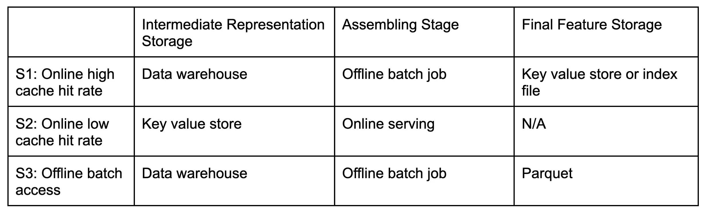
S1 typically corresponds to ranking candidate features, such as total number of views a Snap Discover channel gets. Each candidate could be ranked in different requests and each request will score against many candidates. It makes sense to assemble the blocks offline. The final features can be pushed to a key value store or document index for serving.
S2 is suitable for low cache hit rate or smaller scale use cases. We directly query the intermediate representations from a key-value store and assemble in the online serving path.
S3 supports the so-called point-in-time lookup. This happens in offline feature generation pipelines, where the inputs are impressions that we will train on and we need to compute the feature values associated with the impressions at serving time. This is a challenging task. In the next section we will talk about how this works.
During online scoring, we always fetch the latest feature values available from the feature store. If we are to generate the feature values offline, we need to reproduce the same data as online. Otherwise we will introduce online and offline data discrepancy.
One naive way is to log a timestamp that indicates when we fetch the features online. If we have a table that keeps track of the feature values at every possible timestamp, we can look up the value. However, this is infeasible for near-real time features at snap scale. Imagine if you have 100M keys and support one-minute granularity. That’s 100M * 60 * 24 * 30 = 4320 billion keys for 30 days. Additionally, you need to calculate feature value for most of the 100M keys each minute for sliding window aggregations.
We take advantage of the associative and commutative nature of the aggregations to make this work. As mentioned earlier, we store the representation blocks for various intervals in Apache Iceberg. For example:
These pre-aggregated stats are partitioned by primary key and time bucket.
When generating features offline, the input is a collection of rows containing the impression time, feature version pointer, look up keys(e.g. snap id, user id etc) and other data. The feature version pointer is logged when we fetch the features online and indicates the latest time bucket that has been ingested into the online DB. Since the offline data warehouse contains the same data as online, by limiting the largest time bucket used for feature computation we can match the online behavior.
Assume for now the input data primary key sharding matches with the sharding of the pre-aggregated stats(shuffle is required if not). To scale out the work, we break it down into many work items by shards and impression time range. Each work item therefore only needs to run iceberg queries to load a single shard and the matching aggregation intervals. For example, if the impression time range is May 31 12am to 11pm, to calculate 30-day counters with 12hr and 1hr granularities, we load:
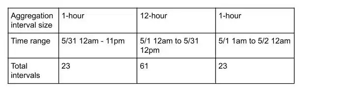
After loading the data, we put them into an in-memory map keyed by the primary key. There’s an aggregator per feature per key to combine the stats. Since we repeatedly need to look up a range of aggregation intervals per impression, we use a binary search tree to speed up the time range query. After the worker processes all the iceberg data, it calls the finalize method to extract the features. Figure 4 illustrates this process.
Compared to the naive approach, we utilize in memory maps local to each shard. And since we work with intermediate blocks, we don’t need to calculate the final feature value all the time.
One common question that arises in data processing systems is how to accommodate backfilled data. There are two main methodologies:
Copy on write. Load the original file, make modifications and replace.
Merge on read. Create new files for the new data and merge old and new records at read time.
Robusta uses merge on read since it works better for the feature backfilling use case:
When backfilling features, we need to touch all the files. Rewriting all the data each time is not practical given that experimenting with new features is a high frequency activity.
Since most of the backfilling is creating brand-new columns, we are not reducing the amount of data to load on the read path even if we combine the data at write time. The major downside for merge on read is smaller files to load, which isn’t too fatal and can be solved by periodic consolidation jobs or batching multiple backfills at a time.
It’s fairly cheap to merge data in memory on the read path given we already load all the relevant data for a particular shard.
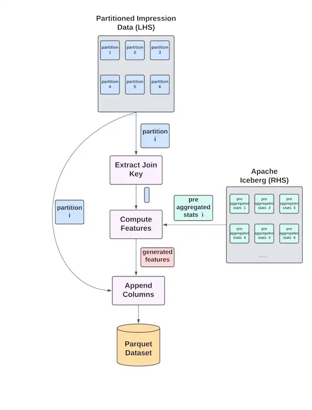
Offline generated features need to be joined with features from other sources before they can be fed into the model. For example, we might have impression data and logged features on the left hand side(LHS) and offline generated features on the right hand side(RHS). The interesting thing about the join is that the RHS is computed per partition on demand(see above section). This naturally fits well with bucketed joins.
Robusta feature computation requires the input data partitioning to be aligned with the pre-aggregated stats in Iceberg. To reduce data shuffling, we enforce consistent user id partitioning to both LHS and RHS. At join time, each worker simply loads the relevant join keys from the LHS for a single partition to compute the user features(figure 5). For non-user features, we do need to shuffle the LHS look up keys to align the partitioning. Once the features are produced, we shuffle them again to match the LHS partitioning on user ids.
The output results are parquet files. We ensure the generated feature rows follow the exact same order as input data within a partition. We make use of the columnar format and implement a custom parquet writer to directly append the generated columns to the original LHS columns, avoiding the need to load all LHS columns into memory and combine.
When we free MLEs from having to touch online systems or wait for feature logs, we observe significant acceleration in the creation of new features. Customer teams at Snap gain access to more advanced functionalities such as sparse id list features [8], long aggregation windows or near-real time features, etc.
The launch of Robusta has produced many impactful features and brought sizable business gain. As a result, we are continuing to put strong emphasis on enabling easy feature experimentation for other types of features, in addition to aggregation features.
[1] Zipline: Airbnb’s Machine Learning Data Management Platform
[2] Michelangelo Palette: A Feature Engineering Platform at Uber
[3] Point-in-Time Correctness in Real-Time Machine Learning
[4] MapReduce: Simplified Data Processing on Large Clusters
[6] Apache Spark
[7] Apache Iceberg
[8] Deep Neural Networks for YouTube Recommendations.
P. Covington, J. Adams, and E. Sargin. RecSys , page 191-198. ACM, (2016)